Code
library(pacman)
pacman::p_load(tidyverse, sf, dplyr, rnaturalearth, showtext, ragg, glue)
showtext_auto()library(pacman)
pacman::p_load(tidyverse, sf, dplyr, rnaturalearth, showtext, ragg, glue)
showtext_auto()# get south america polygon
sa <- ne_countries(continent = "South America", returnclass = "sf") |>
st_union() |> # single polygon
st_transform(3857) # project to meters for equal grid spacing
# create a regular grid of points
grid_spacing <- 60000 # in meters; smaller = denser grid
grid <- st_make_grid(sa,
what = "centers",
cellsize = grid_spacing) |>
st_as_sf() |>
st_intersection(sa) # keep only points inside polygon# color pallete
set.seed(123)
golden_palette <- c("#F9C74F", "#F8961E", "#F3722C", "#F9844A")
grid$color <- sample(golden_palette, nrow(grid), replace = TRUE)
grid$y <- st_coordinates(grid)[, 2]ggplot() +
geom_sf(data = grid, aes(color = y), size = 0.8, show.legend = FALSE) +
scale_color_gradientn(colors = golden_palette) +
coord_sf(expand = FALSE, clip = "off") +
theme_void() +
theme(
plot.background = element_rect(fill = "white", color = NA),
plot.margin = margin(t = 0, # Top margin
r = 1, # Right margin
b = 0, # Bottom margin
l = 1, # Left margin
unit = "cm")) 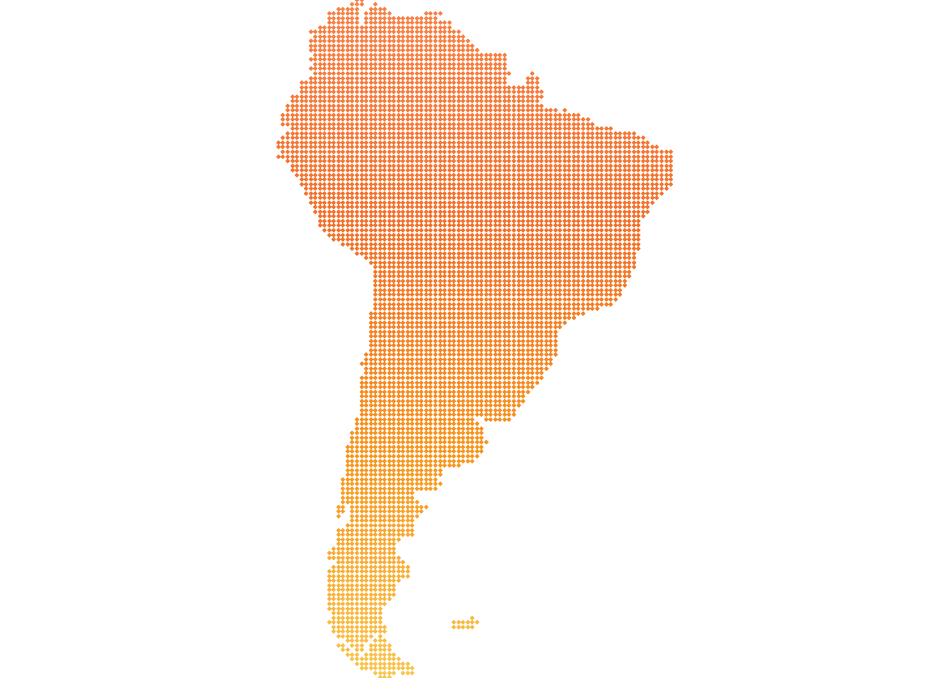
Last few tweaks made on Canva
