The goal is to analyze Netflix’s content strategy to understand how various factors like content type, language, release season, and timing affect viewership patterns. By identifying the best-performing content and the timing of its release, the aim is to uncover insights into how Netflix maximizes audience engagement throughout the year.
Objectives
The primary goal is to analyze Netflix’s content strategy across multiple dimensions:
Content Performance: Compare viewership patterns between movies and TV shows
Language Impact: Understand how language affects global viewership
                                     Title Available.Globally. Release.Date
1                The Night Agent: Season 1                 Yes   2023-03-23
2                Ginny & Georgia: Season 2                 Yes   2023-01-05
3 The Glory: Season 1 // 더 글로리: 시즌 1                 Yes   2022-12-30
4                      Wednesday: Season 1                 Yes   2022-11-23
5      Queen Charlotte: A Bridgerton Story                 Yes   2023-05-04
6                            You: Season 4                 Yes   2023-02-09
  Hours.Viewed Language.Indicator Content.Type
1 81,21,00,000            English         Show
2 66,51,00,000            English         Show
3 62,28,00,000             Korean         Show
4 50,77,00,000            English         Show
5 50,30,00,000            English        Movie
6 44,06,00,000            English         Show
Data Processing Pipeline
Upon initial assessment, there are some data cleaning steps necessary.
There are some interesting things to notice, namely, the p#c1071eominance of TV shows spoken in English, with the exception of two very high placed Korean pieces. Next, I will take a look into the language distribution of Netflix releases.
Language Analysis
Code
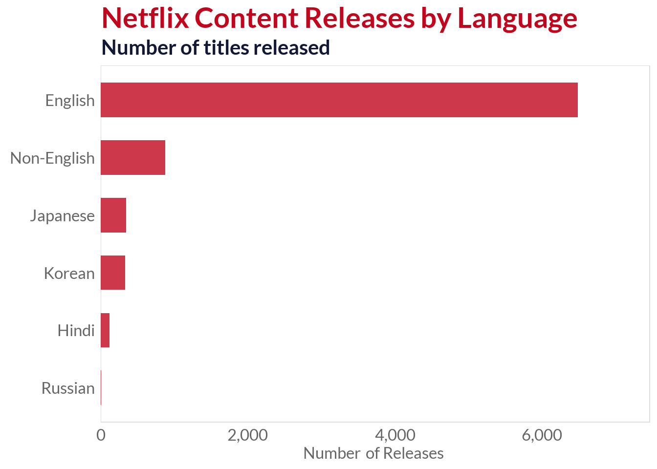
language_summary <- netflix_clean %>%group_by(Language.Indicator) %>%summarise(Count =n(),Total_Hours =sum(Hours.Viewed),Avg_Hours =mean(Hours.Viewed),Median_Hours =median(Hours.Viewed),.groups ='drop' ) %>%arrange(desc(Count)) %>%mutate(Language_Label =case_when( Language.Indicator =="English"~"English", Language.Indicator =="Non-English"~"Non-English",TRUE~ Language.Indicator ),# Calculate percentage of total releasesPercentage =round(Count /sum(Count) *100, 1) )# Graph showing number of releases by languageggplot(language_summary, aes(x =reorder(Language_Label, Count), y = Count)) +geom_col(fill ="#c1071e", alpha =0.8, width =0.6) +coord_flip() +scale_y_continuous(labels =comma_format(), expand =expansion(mult =c(0, 0.15))) +labs(title ="Netflix Content Releases by Language",subtitle ="Number of titles released",x =NULL,y ="Number of Releases", ) +theme()
So, we can see that English-speaking releases dominate the market. Of non-English languages, Japanese and Korean releases are the most common. The success of Korean releases (being two out of the five most watched pieces) shows a strong trend and preference for Korean made movies and TV shows.
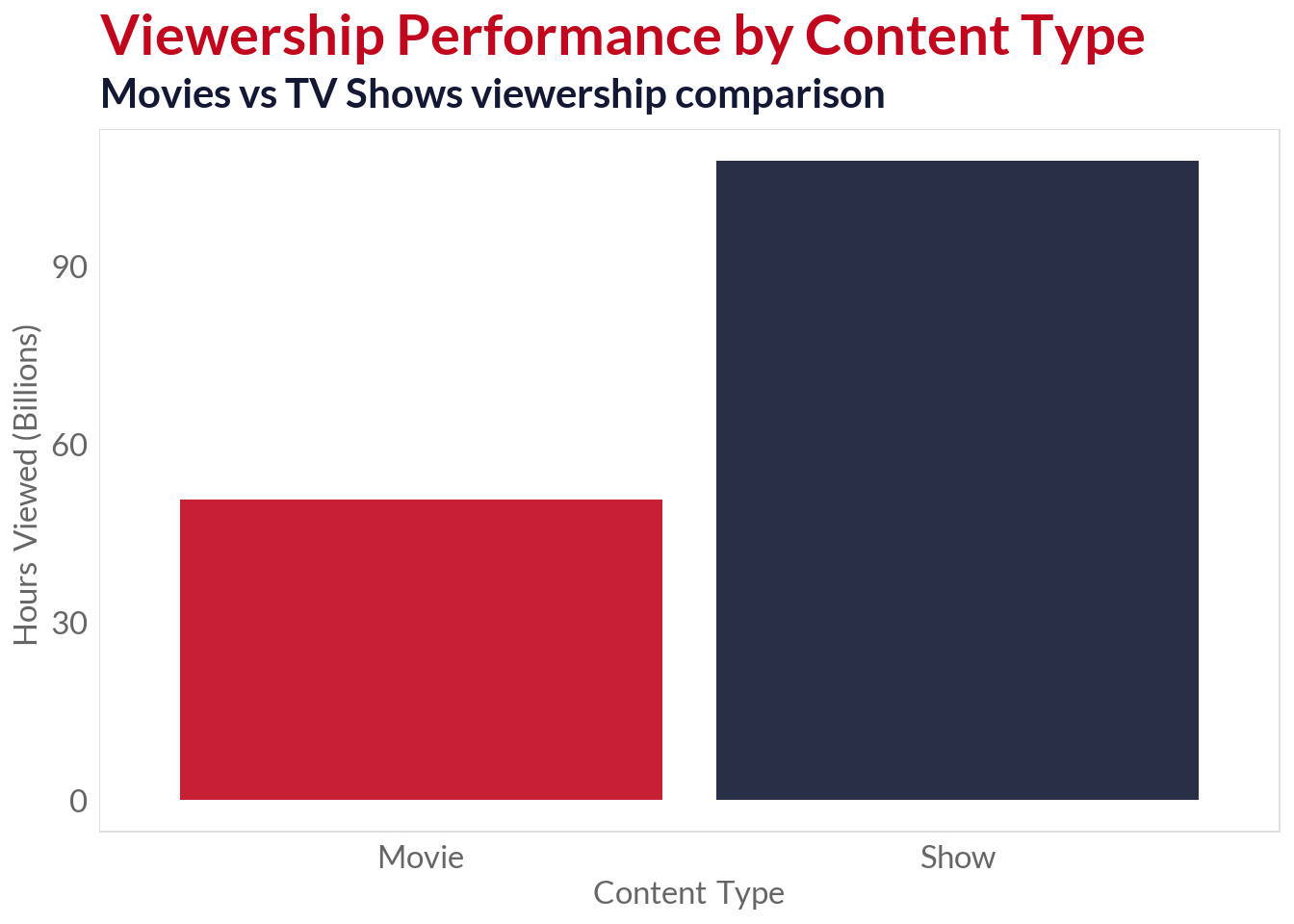
ggplot(netflix_data, aes(x = Content.Type, y = Hours.Viewed, fill = Content.Type)) +geom_col(alpha =0.9) +scale_fill_manual(values =c("#c1071e", "#131834")) +scale_y_continuous(labels =label_number(scale =1e-9)) +labs(title ="Viewership Performance by Content Type",subtitle ="Movies vs TV Shows viewership comparison",x ="Content Type",y ="Hours Viewed (Billions)" ) +theme(legend.position ="none")
Thus:
Movies had more titles produced (14 104), but lower individual performance
TV shows had less titles produced (10 708), but very high individual performance
Average viewership: Shows get ~2.8x more views than movies (100.6M vs 35.9M hours)
Median viewership: Shows get ~2.5x more views than movies (87.2M vs 35.5M hours)
Total viewership: Despite fewer titles, shows generate ~1.5x more total hours (708B vs 450B)
So, I infer the following strategic implications:
Content Investment Strategy: TV shows demonstrate superior ROI in terms of viewer engagement per title
Portfolio Balance: While movies provide content volume, TV shows drive sustained engagement
Resource Allocation: The data suggests prioritizing TV show development for maximum viewership impact
Temporal Analysis
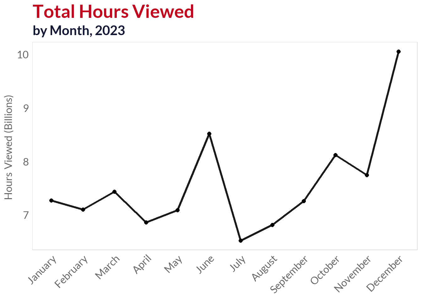
Utilizing the new variables created in the data processing step, I will visualize how the amount of hours watched distribute in time to infer whether or not there is a relationship between the month, quarter or day of the week a new product is released and the engagement it receives.
Quarter 4 (Oct-Dec) emerges as the optimal release window, generating the highest total viewership
Quarter 1 (Jan-Mar) shows strong performance, likely capitalizing still capitalizing on holidays
Quarters 2 and 3 (Apr-Sep) demonstrate relatively lower engagement, suggesting seasonal viewing patterns where audiences may be more occupied with summer (northern hemisphere) and mid-year vacations (southern hemisphere)
Strategic Timing: The data reveals a clear seasonal strategy where Netflix concentrates high-impact releases during periods of maximum audience availability, particularly leveraging the winter months for premium content launches
The performance gap widens in Q4, suggesting strong demand for binge-worthy series during holiday periods
The best months for releasing high-impact shows are October and November
Conclusion
This analysis demonstrates how language, content type, and release timing influence Netflix viewership. Based on the findings, I recommend the following:
Invest Heavily in TV Shows: Given their higher ROI, prioritize show development over films.
Capitalize on Q4 & Q1 Windows: Maximize releases during Oct–Mar when engagement peaks.
Expand Successful Non-English Offerings: Korean content, despite lower volume, has outsized performance.