Dungeons and Dragons is a role-playing game which almost all gameplay aspects comes down to rolling die – for combat, skills checks, or even during conversations with NPCs. In this post, we will look into concepts of probability applied to the Dungeons & Dragons gameplay.
The Basics: Simple Die Rolls
The twenty-sided-die, also known as d20, is a staple for the game and the one the player uses the most during their campaign.
In probability theory, a sample space is the set of all possible outcomes for an experiment. For a standard twenty-sided die (d20), our sample space is simply the integers from 1 to 20. Each outcome has an equal probability of occurring, which we call a uniform distribution.
The probability of any specific outcome on a fair d20 is: P(rolling any specific number) = 1/20 = 0.05 or 5%
Likewise, if you need to roll a 15 or higher, your chances are: P(15 or 16 or 17 or 18 or 19 or 20) = 6/20 = 0.30 or 30%
Simulating Die Rolls with R
Code
# Simulate a single d20 rollsingle_roll <-sample(1:20, 1)print(single_roll)
[1] 11
Code
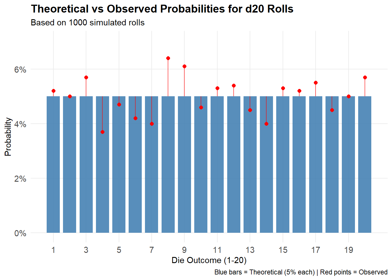
# Simulate multiple rolls to see the patternn_rolls <-1000rolls <-sample(1:20, n_rolls, replace =TRUE)# Calculate the frequency of each outcomeroll_table <-table(rolls)# Convert to probabilitiesroll_probabilities <- roll_table / n_rollsprint(roll_probabilities)
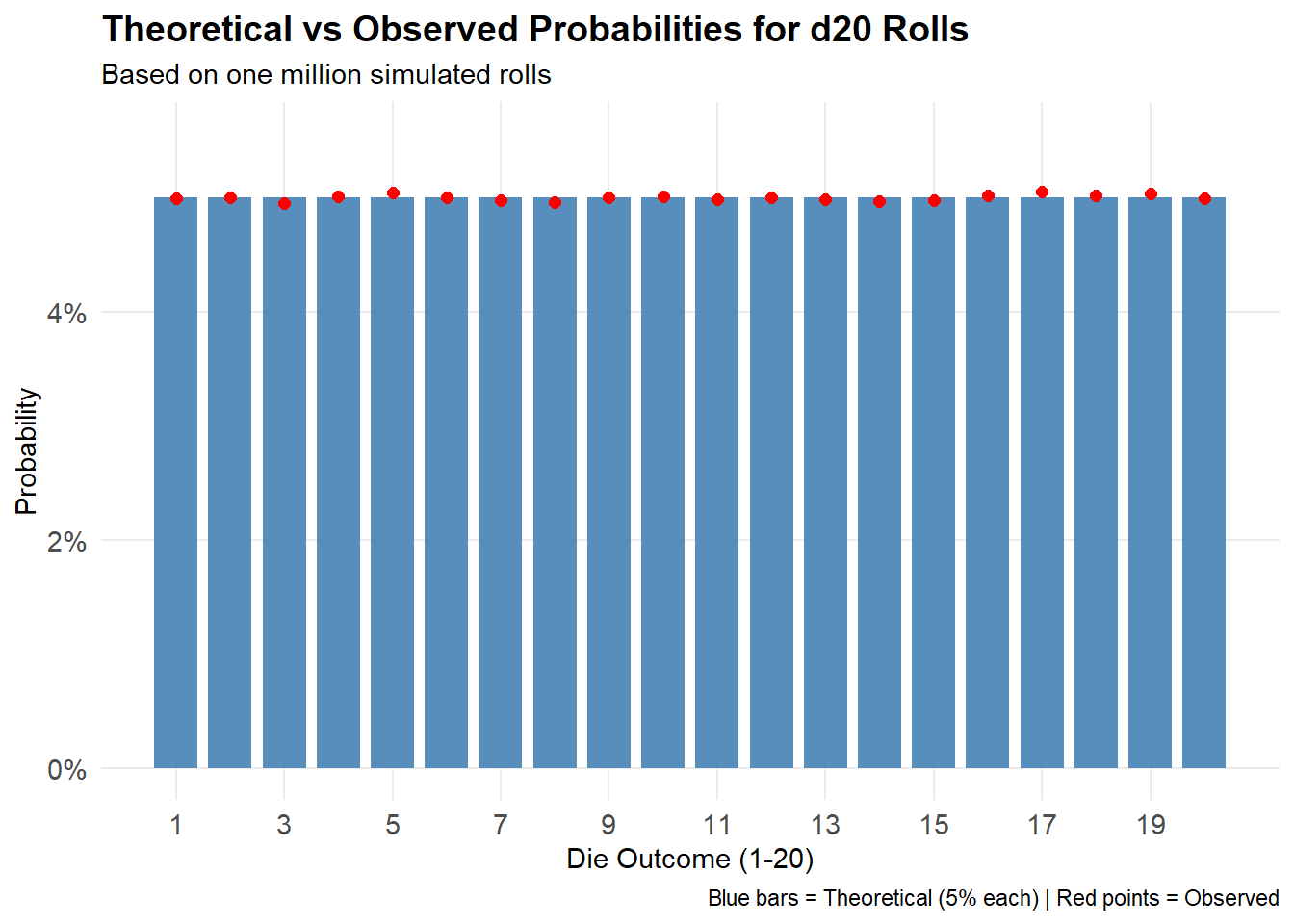
Close enough to those 0.05%! The beauty of running many simulations is that with enough rolls we can observe frequencies very close to the theoretical approach. To illustrate, let’s simulate rolling one million d20s.
n_rolls <-1000000rolls <-sample(1:20, n_rolls, replace =TRUE)roll_table <-table(rolls)roll_data <-data.frame(outcome =1:20,theoretical_prob =rep(1/20, 20) # 5% for each outcome)roll_data$observed_freq <-sapply(1:20, function(x) {if (as.character(x) %in%names(roll_table)) {return(as.numeric(roll_table[as.character(x)])) } else {return(0) }}) # simulate observed frequencies roll_data$observed_prob <- roll_data$observed_freq / n_rolls # freq to probggplot(roll_data, aes(x = outcome)) +geom_col(aes(y = theoretical_prob), alpha =0.9, fill ="steelblue", width =0.8) +geom_point(aes(y = observed_prob), color ="red", size =2) +geom_segment(aes(xend = outcome, y = theoretical_prob, yend = observed_prob),color ="red", alpha =0.7) +scale_x_continuous(breaks =seq(1, 20, 2)) +scale_y_continuous(labels = scales::percent_format(accuracy =1),limits =c(0, max(c(roll_data$theoretical_prob, roll_data$observed_prob)) *1.1)) +labs(title ="Theoretical vs Observed Probabilities for d20 Rolls",subtitle =paste("Based on one million simulated rolls"),x ="Die Outcome (1-20)",y ="Probability",caption ="Blue bars = Theoretical (5% each) | Red points = Observed") +theme_minimal() +theme(panel.grid.minor =element_blank(),plot.title =element_text(size =14, face ="bold"),axis.text =element_text(size =11))
Recapitulating:
With enough rolls, the observed frequencies approach the theoretical 5% for each outcome. This is illustrated by our one million simulations graph
In small samples, you might see significant deviations from the expected frequencies, as we see in the 1000 simulations graph
Each roll is independent. Rolling three 1s in a row doesn’t make a 20 more likely on the next roll.
We can also create a function to calculate the probability of rolling equal or higher than k on any dice.
Code
# Function to calculate probability of rolling at or above a targetprob_at_least <-function(target, die_size =20) {if (target > die_size) return(0)if (target <=1) return(1) favorable_outcomes <- die_size - target +1 probability <- favorable_outcomes / die_sizereturn(probability)}prob_at_least(15, 20) # 30% chance of rolling 15+ on d20
[1] 0.3
Code
prob_at_least(4, 6) # 50% chance of rolling 4+ on d6
[1] 0.5
If you want to calculate the probability of getting exactlyk:
Advanced Roleplaying: Advantage and Advantange/Disadvantage Rolls
Once we move beyond single die rolls, the probability landscape becomes much more interesting. D&D’s advantage and disadvantage mechanics, different dice combinations for damage, and the concept of probability distributions all come into play when we start rolling multiple dice.
Understanding Advantage and Disadvantage Rolls
Advantage and Disadvantage rolls debuted in D&D 5e. Instead of adding your characters ability modifier to your roll, there are situations (either very good or very bad) where your DM may ask you to roll twice and take the higher (advantage) or lower (disadvantage) result. But how much does this actually change your odds?
The Maths of Advantage
When you roll with advantage, you’re looking for the probability that at least one of your two d20 rolls meets or exceeds your target. This is easier to calculate using the complement rule:
P(success with advantage) = 1 - P(both rolls fail)
P(both rolls fail) = P(first roll fails) × P(second roll fails)
Code
library(knitr)# Function to calculate advantage probabilityprob_advantage <-function(target, die_size =20) { prob_single_fail <- (target -1) / die_size prob_both_fail <- prob_single_fail^2 prob_advantage <-1- prob_both_failreturn(prob_advantage)}# Function to calculate disadvantage probability prob_disadvantage <-function(target, die_size =20) { prob_single_success <- (die_size - target +1) / die_size prob_both_success <- prob_single_success^2 prob_disadvantage <- prob_both_successreturn(prob_disadvantage)}# Compare normal vs advantage vs disadvantage for different DCstargets <-seq(5, 20, 1)normal_probs <-sapply(targets, prob_at_least)advantage_probs <-sapply(targets, prob_advantage)disadvantage_probs <-sapply(targets, prob_disadvantage)# Create comparison data framecomparison_data <-data.frame(DC = targets,Normal =round(normal_probs, 4),Advantage =round(advantage_probs, 4),Disadvantage =round(disadvantage_probs, 4))kable(comparison_data, caption ="Success Probabilities: Normal vs Advantage vs Disadvantage",digits =4)
Success Probabilities: Normal vs Advantage vs Disadvantage
DC
Normal
Advantage
Disadvantage
5
0.80
0.9600
0.6400
6
0.75
0.9375
0.5625
7
0.70
0.9100
0.4900
8
0.65
0.8775
0.4225
9
0.60
0.8400
0.3600
10
0.55
0.7975
0.3025
11
0.50
0.7500
0.2500
12
0.45
0.6975
0.2025
13
0.40
0.6400
0.1600
14
0.35
0.5775
0.1225
15
0.30
0.5100
0.0900
16
0.25
0.4375
0.0625
17
0.20
0.3600
0.0400
18
0.15
0.2775
0.0225
19
0.10
0.1900
0.0100
20
0.05
0.0975
0.0025
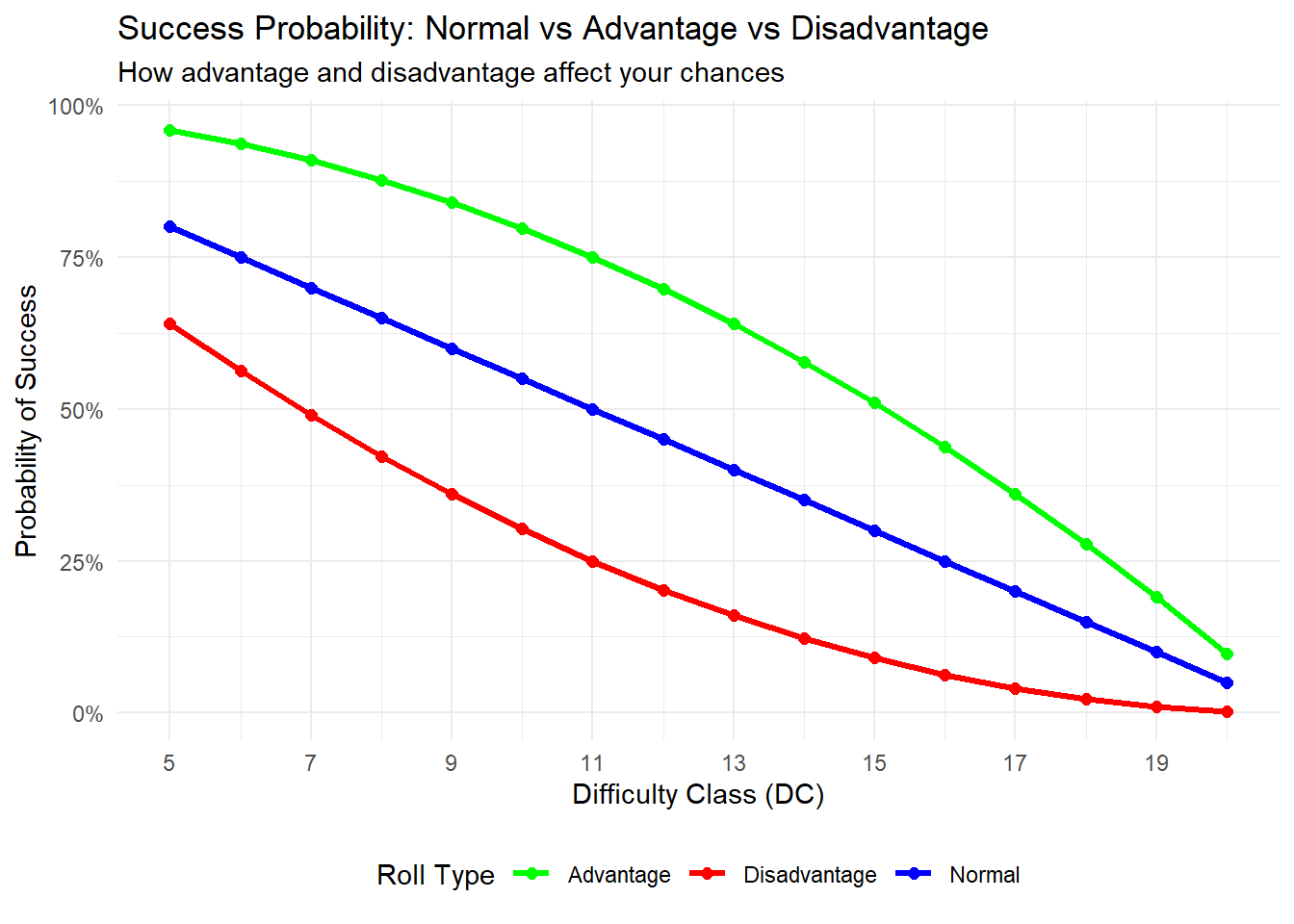
As we can see, rolling with advantage significantly increases our chances of rolling a high number, while disadvantage increases the odd of rolling low numbers. Now, onto visualizing:
Code
library(tidyr)library(tidyverse)# Reshape data for plottingplot_data <- comparison_data %>%pivot_longer(cols =c(Normal, Advantage, Disadvantage),names_to ="roll_type", values_to ="probability")ggplot(plot_data, aes(x = DC, y = probability, color = roll_type)) +geom_line(size =1.2) +geom_point(size =2) +scale_color_manual(values =c("Normal"="blue", "Advantage"="green", "Disadvantage"="red")) +scale_y_continuous(labels = scales::percent_format(accuracy =1)) +scale_x_continuous(breaks =seq(5, 20, 2)) +labs(title ="Success Probability: Normal vs Advantage vs Disadvantage",subtitle ="How advantage and disadvantage affect your chances",x ="Difficulty Class (DC)",y ="Probability of Success",color ="Roll Type") +theme_minimal() +theme(legend.position ="bottom")
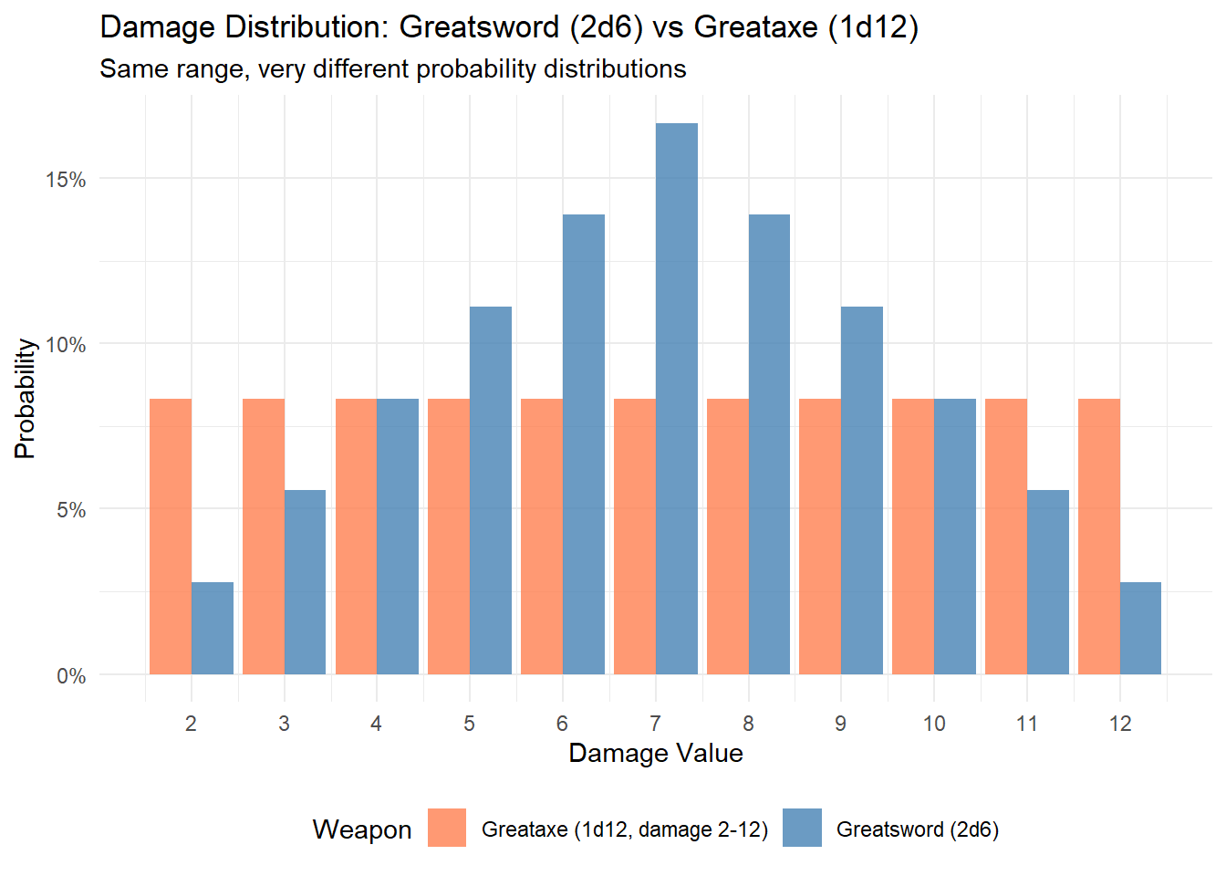
Damage Types: What is the difference between 2d6s and 1d12?
Another common D&D scenario involves different damage dice combinations. For example, a greatsword can deal 2d6 damage, while a greataxe deals 1d12. Both have the same range (2-12 vs 1-12), but very different probability distributions.
Code
# Simulate damage rollsn_simulations <-10000# 2d6 (greatsword) - roll two d6 and sumdamage_2d6 <-replicate(n_simulations, sum(sample(1:6, 2, replace =TRUE)))# 1d12 (greataxe) - roll one d12 damage_1d12 <-sample(1:12, n_simulations, replace =TRUE)# Calculate theoretical probabilities for 2d6theoretical_2d6 <-sapply(2:12, function(x) {# Count ways to make sum x with 2d6 ways <-0for(i in1:6) {for(j in1:6) {if(i + j == x) ways <- ways +1 } }return(ways /36) # 36 total outcomes for 2d6})# Create comparison datadamage_comparison <-data.frame(damage =2:12,theoretical_2d6 = theoretical_2d6,observed_2d6 =sapply(2:12, function(x) sum(damage_2d6 == x) / n_simulations),theoretical_1d12 =rep(1/12, 11), # outcomes 2-12 for fair comparisonobserved_1d12 =sapply(2:12, function(x) sum(damage_1d12 == x) / n_simulations))# Add damage 1 for 1d12 (greatsword can't roll 1)damage_1d12_full <-data.frame(damage =1:12,prob_1d12 =rep(1/12, 12))kable(damage_comparison,caption ="Damage Comparison",digits =4)