Code
library(pacman)
pacman :: p_load(tidytuesdayR, tidyverse, dplyr, janitor, ggtext, showtext, scales, glue, marquee)

tuesdata <- tidytuesdayR::tt_load('2025-11-18')This week challenge dataset in on Sherlock. Check the TidyTuesday GitHub repo for the data.
library(pacman)
pacman :: p_load(tidytuesdayR, tidyverse, dplyr, janitor, ggtext, showtext, scales, glue, marquee)
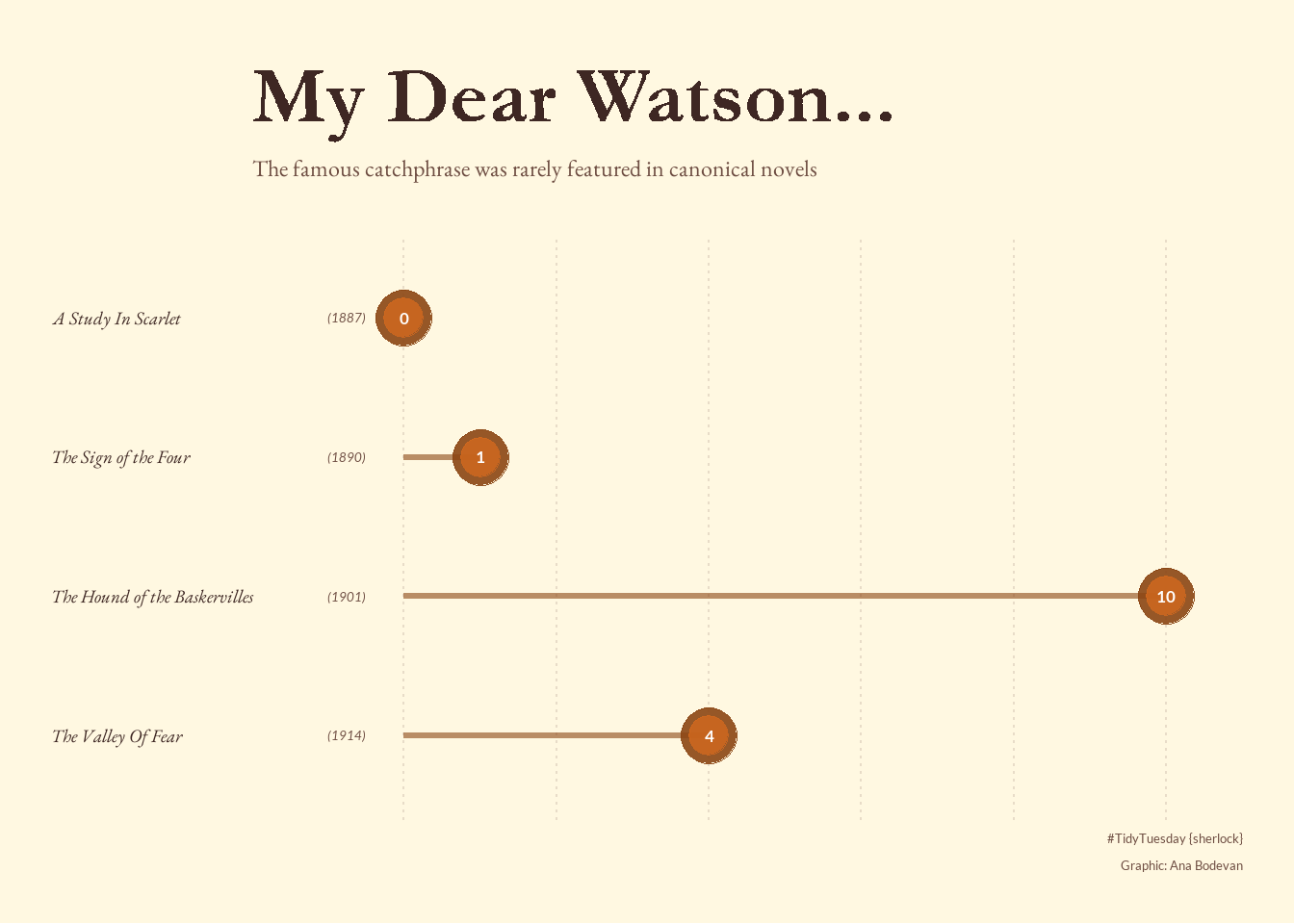
tuesdata <- tidytuesdayR::tt_load('2025-11-18')There are four canonical Sherlock Holmes novels: A Study in Scarlet, The Sign of the Fours, The Hound of Baskervilles and The Valley of Fear
holmes <- tuesdata$holmes

novels <-
  tribble(
    ~book,~year,
    "A Study In Scarlet",1887,
    "The Sign of the Four",1890,
    "The Hound of the Baskervilles",1901,
    "The Valley Of Fear",1914
)lines <-
holmes |>
filter(book %in% novels$book) |>
left_join(novels) |>
drop_na(text) |>
arrange(year) |>
mutate(watson = str_detect(text, "[Mm]y dear Watson"))
watson_counts <-
lines |>
group_by(book, year) |>
summarize(count = sum(watson), .groups = "drop") |>
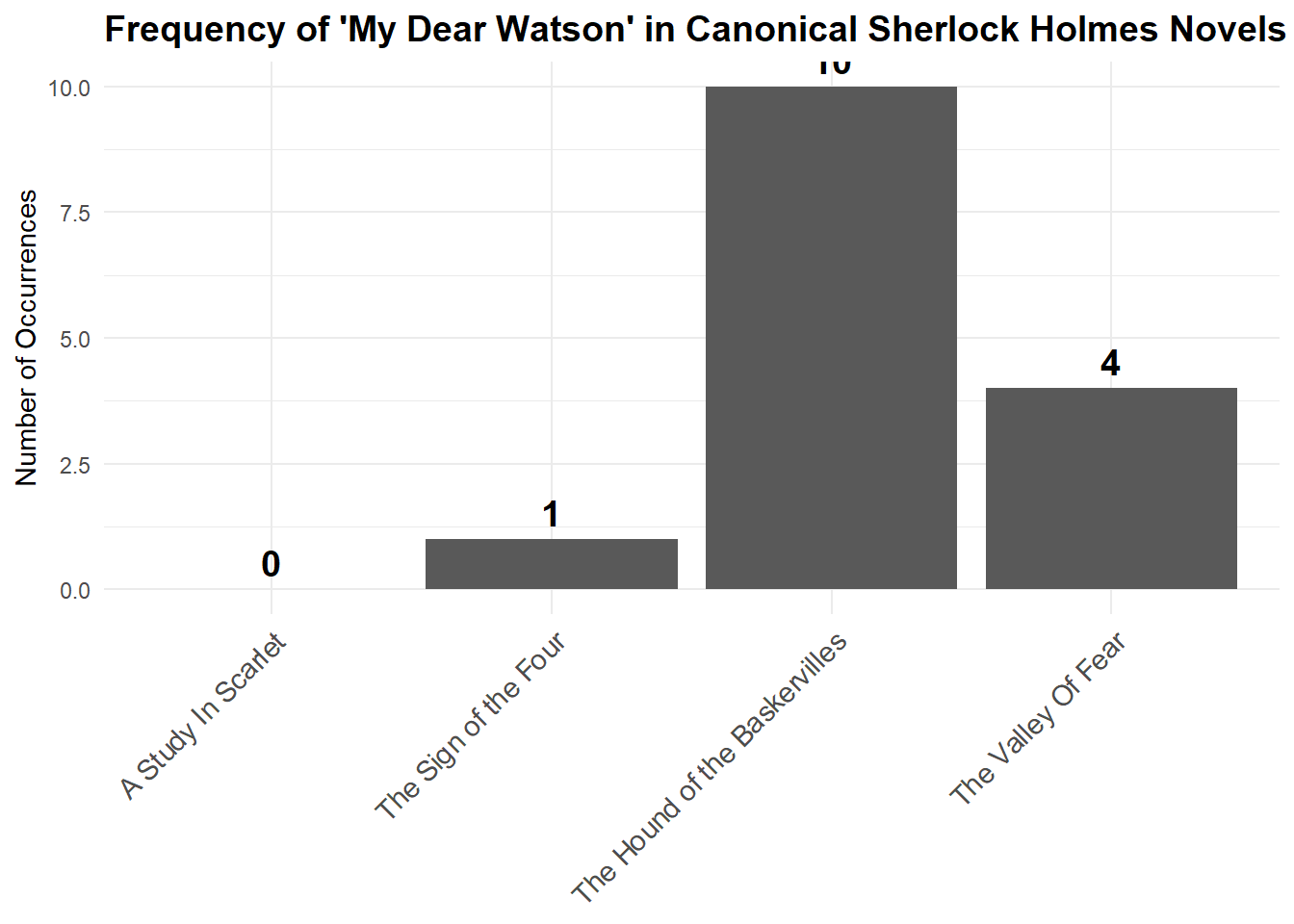
arrange(year)ggplot(watson_counts, aes(x = reorder(book, year), y = count)) +
geom_col() +
geom_text(aes(label = count), vjust = -0.5, size = 5, fontface = "bold") +
labs(
title = "Frequency of 'My Dear Watson' in Canonical Sherlock Holmes Novels",
x = NULL,
y = "Number of Occurrences"
) +
theme_minimal() +
theme(
axis.text.x = element_text(angle = 45, hjust = 1, size = 11),
plot.title = element_text(face = "bold", size = 14)
)
font_add_google("EB Garamond", "garamond")
font_add_google("Lato", "lato")
showtext_auto()# Create dot plot
ggplot(watson_counts, aes(x = count, y = reorder(book, -year))) +
# Segment from y-axis to point
geom_segment(aes(x = 0, xend = count, y = book, yend = book),
color = "#8B4513", linewidth = 1.2, alpha = 0.6) +
# Dots
geom_point(size = 10, color = "#8B4513", alpha = 0.9) +
geom_point(size = 7, color = "#D2691E", alpha = 0.8) +
# Count labels inside dots
geom_text(aes(label = count), color = "white", size = 4.5,
fontface = "bold", family = "lato") +
# Year labels after book titles
geom_text(aes(label = paste0("(", year, ")"), x = -0.5),
hjust = 1, size = 3.5, color = "#6D4C41",
family = "lato", fontface = "italic") +
# Styling
scale_x_continuous(breaks = seq(0, 10, 2),
limits = c(-2, 11),
expand = c(0, 0)) +
labs(
title = "**My Dear Watson...**",
subtitle = "The famous catchphrase was rarely featured in canonical novels",
caption = "#TidyTuesday {sherlock}\nGraphic: Ana Bodevan",
x = NULL,
y = NULL
) +
theme_void(base_family = "garamond") +
theme(
plot.title = element_marquee(
family = "garamond",
size = 32,
color = "#3E2723",
margin = margin(b = 5)
),
plot.subtitle = element_text(
size = 18,
family = "garamond",
color = "#6D4C41",
margin = margin(b = 20, t=2)
),
plot.caption = element_text(size = 10, family = "lato", color = "#6D4C41"),
plot.background = element_rect(fill = "#FFF8E1", color = NA),
panel.background = element_rect(fill = "#FFF8E1", color = NA),
panel.grid.major.y = element_blank(),
panel.grid.minor = element_blank(),
panel.grid.major.x = element_line(color = "#E8DCC8", linewidth = 0.4, linetype = "dotted"),
axis.text.y = element_text(size = 14, color = "#3E2723",
hjust = 0, face = "italic"),
axis.text.x = element_blank(),
axis.ticks = element_blank(),
plot.margin = margin(20, 20, 20, 20)
)